Note: The R-version of this tutorial (not replicating the same result) can be found at https://sites.uab.edu/jayzhanglab/ai-pipeline-r/.
I.Overview
This tutorial demonstrates how to use Autoencoder, Sparse model analysis, and semi-supervised learning to analyze single-cell RNA sequencing (scRNAseq) data. Autoencoder is to embed and cluster the cells, and may be repeated multiple times to see novel/interested cell clusters. Sparse model analysis can be used to perform pathway/gene set enrichment analysis, and can also ‘quantify’ the activity of a specific pathway among cell groups. Semi-supervised learning may infer how a specific cell cluster transit to other cell clusters, given that the real-time order is known.
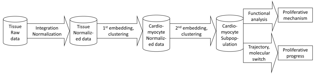
The overall pipeline steps are according to figure 1. It includes
– Data normalization (strongly recommended using Seurat). Also, cell group (sample ID) and expression matrix files need to be processed and slightly formatted
– Cell clustering, embedding, and finding cluster markers. Usually, the first round separates the cell types; then the second and following rounds may identify cell type subpopulations.
– Pathway/geneset enrichment analysis, by Sparse model or marker-based method (i.e. DAVID) – Trajectory analysis can be applied when interesting clusters and time-course information appear.
The dataset used in this tutorial is from https://www.ncbi.nlm.nih.gov/geo/query/acc.cgi?acc=GSE185289. This tutorial only uses the following heart:
Fetal: embryonic day 80 heart. Highly proliferative cardiomyocytes. The code and data for this tutorial can be downloaded at https://uab.box.com/s/0g6r0mauohupfi5e6upxuj3sd7xcfvs6.
CTL-P56: wildtype heart, postnatal day 56. Cardiomyocyte proliferation is virtually 0.
AR1-P28: heart underwent apical resection on neonatal day1, then completely recovered on postnatal day 28
AR1-MI28-P30: heart underwent apical resection on neonatal day1, then the second LAD ligation on day 28. The tissue was collected on postnatal day 30 (2 days after the second injury). It would also completely recover. Cardiomyocytes are expected to proliferate for remuscularization.
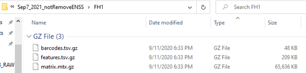
MI28-P30: heart only underwent second LAD ligation on day 28, which would not recover (fibrotic). The tissue was collected on postnatal day 30 (2 days after the second injury). Cardiomyocytes are less proliferative. The raw data, in 10XGenomic format, are supposed to be in the ’10XFormat’ folder. Each group (sample) should have its own subfolder. The 10X format has three files: ‘bardcodes.csv.gz’, ‘features.tsv.gz’, and matrix.mtx.gz’ for each group/sample. For example
II. Data normalization (R/Seurat)
In many cases, Seurat normalization processes the data very well prior to embedding/clustering by Autoencoder. A good Seurat tutorial could be found at https://satijalab.org/seurat/articles/pbmc3k_tutorial.html. The R-Seurat example, which was tested in R version 4.0.3, is below
Step 0: Install the required library (Seurat, sctransform, and Matrix), if needed. Then load them
# install seurat if needed
#install.packages("Seurat")
#if (!requireNamespace("BiocManager", quietly = TRUE))
#  install.packages("BiocManager")
#BiocManager::install("multtest")
library(Seurat)
library(sctransform)
library("Matrix")
Step 1: Import the scRNA data after processed by Cell Ranger. Here we have 5 groups. We would import each group one by one, then merge them into a ‘seuratObj’
Data <- Read10X(data.dir = "10XFormat/Fetal"); seuratObj <- CreateSeuratObject(counts = Data)
Data <- Read10X(data.dir = "10XFormat/CTL-P56");  seuratObj2 <- CreateSeuratObject(counts = Data)
Data <- Read10X(data.dir = "10XFormat/AR1-P28");  seuratObj3 <- CreateSeuratObject(counts = Data)
Data <- Read10X(data.dir = "10XFormat/AR1-MI28-P30");  seuratObj4 <- CreateSeuratObject(counts = Data)
Data <- Read10X(data.dir = "10XFormat/MI28-P30");  seuratObj5 <- CreateSeuratObject(counts = Data)
seuratObj <- merge(seuratObj, y = c(seuratObj2, seuratObj3, seuratObj4, seuratObj5), add.cell.ids = dataID)
rm(seuratObj2); rm(seuratObj3); rm(seuratObj4); rm(seuratObj5); # remove the other 'seuratObj' to free memory
The quality control steps, including removing cells having a high percentage of mitochondrial transcript and doublet detection, are strongly recommended. They are skipped in this tutorial because the data are already processed. See https://satijalab.org/seurat/articles/pbmc3k_tutorial.html for more details in quality controls.
Step 2: Normalize the data with Seurat. This tutorial does not use Seurat’s SCTransform function
seuratObj <- NormalizeData(seuratObj, normalization.method = "LogNormalize", scale.factor = 10000)
seuratObj <- FindVariableFeatures(seuratObj, selection.method = "vst", nfeatures = 2000)
seuratObj <- ScaleData(object = seuratObj, vars.to.regress = c("nCount_RNA", "nFeature_RNA"))
seuratObj <- RunPCA(seuratObj, features = VariableFeatures(object = seuratObj)) # run PCA
seuratObj <- RunUMAP(seuratObj, dims = 1:30, verbose = FALSE) # run Umap
seuratObj <- FindNeighbors(seuratObj, dims = 1:30, verbose = FALSE) # clustering
seuratObj <- FindClusters(seuratObj, verbose = FALSE)
The seuratObj stores the normalization data, which we will need in running Autoencoder.
Step 3: export the normalization results to text file
# export the matrix format to be used by the AI-based pipeline (to be run in Matlab)
writeMM(seuratObj$RNA@data, "NormalizedExpression.txt") # raw transcript count matrix (row: gene, column: cell, in sparse format)
writeMM(seuratObj$RNA@counts, "AdjustedCount.txt") # normalized expression matrix, in sparse format

# export sample ID (required)
sampleID =  seuratObj@assays$RNA@data@Dimnames
sampleID = sampleID[[2]]
df = data.frame(sampleID)
write.csv(df,'sampleID.csv', row.names = FALSE)

# export gene list (required)
geneList = seuratObj@assays$RNA@data@Dimnames
geneList = geneList[[1]]
write.csv(geneList, "filterGeneList.csv")

# export Seurat UMAP in table <cell SampleID+barcode, umap 1 coordinate, umap 2 coordinate>
# this step is optional. We will use Autoencoder UNAP result. But sometimes Seurat UMAP result is useful
umap = seuratObj@reductions$umap
umapCoor = umap@cell.embeddings
df = data.frame(sampleID, umapCoor)
write.csv(df,'SeuratUmapCoor.csv', row.names = FALSE)

# export Seurat cluster in table <cell SampleID+barcode, cluster ID>
# this step is optional. We will use Autoencoder cluster result. But sometimes Seurat cluster result is useful
clusterID = seuratObj@active.ident
clusterID = as.numeric(clusterID)
df = data.frame(sampleID, clusterID)
write.csv(df,'SeuratClusterID.csv', row.names = FALSE)
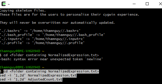
The first two lines in files’ NormalizedExpression.txt’ and ‘AdjustedCount.txt’ should be removed. If these files are small, Notepad++ software (https://notepad-plus-plus.org/downloads/) can easily do so. If these files are large, we might use the ‘sed’ command. This ‘sed’ is built-in Linux, and can be used in Windows after installing Cygwin (see https://cygwin.com/packages/summary/sed-src.html). Open terminal, then run
III. Cluster the cells using Autoencoder (MATLAB)
From this step, the pipeline uses Matlab. This example was tested using Matlab version 2021. It is expected to install at least Matlab’s Neural Network, Deep Learning, and Statistics & Machine Learning toolboxes. Also, the pipeline uses Matlab UMAP https://www.mathworks.com/matlabcentral/fileexchange/71902-uniform-manifold-approximation-and-projection-umap. The necessary files are already in the following folder: https://uab.box.com/s/0g6r0mauohupfi5e6upxuj3sd7xcfvs6. No further installation is needed
Step 1. Prepare the expression matrix to run Autoencoder.
We will use the ‘AdjustedCount.txt’ (raw count, without normalization) to examine which genes are highly expressed (by magnitude) in the data. It is recommended to filter out lowly-expressed genes before using Autoencoder. Which genes and how many genes are used – it is decided case-by-case. For example:
- If comprehensively using the available genes in the data, it will be more accurate and more easily seeing novel (usually small) cell subpopulations. Then, usually the Autoencoder uses ~10,000 genes per cell, might not be able to use Graphic Processing Unit (GPU), and takes ~1day to complete.
- For rapid results, it is recommended to use between 800 and 2000 genes such that the expression matrix and Autoencoder data structure can fit within the GPU memory. The code was tested using a computer having 8GP GPU. To run using GPU, it only uses 878 genes from 39,421 cells. This option is usually chosen in the first clustering round, when we only expect to separate the cell types (i.e. cardiomyocyte from other cardiac cell types).
- Specific gene list. For example, if we want to emphasize cell metabolic, then we might just use genes in ‘Cell metabolic process’ (http://www.informatics.jax.org/vocab/gene_ontology/GO:0044237) to compute the Auntoencoder.
The normalized ‘NormalizedExpression’ will be used to computer Autoencoder. Then, the cells are embedded into ‘cellEncode’, which is the key to visualizing (UMAP) and clustering the cells.
% get the raw transcript count
x = importdata('AdjustedCount.txt');
expressMat = spconvert(x);
save AdjustedCount.mat expressMat -mat; % optional, save the result for future usage
sumExpress = full( sum( expressMat, 2 ) ); % total expression (raw transcript count of each gene), to select the highest expressing genes to
% compute the autoencoder
% get the normalized expression matrix
x = importdata('NormalizedExpression.txt');
expressMat = spconvert(x);
save NormalizedExpression.mat expressMat -mat; % optional, save the result for future usage
autoencoderMat = full( expressMat( find(sumExpress > 40000) , : ) ); % this example use the genes with total expression of 40000 UMI and
% moreto build the autoencoder.
autoenc = trainAutoencoder(autoencoderMat, 'UseGPU', true);% if the autoencoderMat is small enough to fit in the GPU memory, then set 'UseGPU' to true will drastically reduce computing time.% Otherwise, we must set it to false.
cellEncode = encode(autoenc, autoencoderMat); %use autoencoder to embed the cells.
save autoencoderNet.mat autoenc -mat; % optional, save the autoencoder for reusing
save cellEncode.mat cellEncode -mat; % optional, save the cell embeding for reusing
After running, we can see the autoencoder (autoenc) and cells’ encode (cellEncode) in Matlab workspace

Step 2 Identify clusters compute the genes’ statistics in each cluster. The cells are visualized using UMAP
% load the cell sample ID, which is also the cell groups in this analysis
sampleID = readtable('sampleID.csv');
sampleID = table2cell(sampleID(:, 1));
addpath(genpath([pwd, '/MatlabUmap'])); % load the MatlabUmap,
% or simply add all folders and subfolders in MatlabUmap into Matlab Path. See https://www.mathworks.com/help/matlab/ref/addpath.html

[umapCoor, umapStruct, umapCluster] = run_umap(cellEncode');
% umapCoor: umap the 2D embedding (coordinate)
% umapStruct: umap data structure, usually not being used
% umapCluster: the umap Matlab implementation can also perform cell clustering. In some cases, this result is useful.

save umapCoor.mat umapCoor -mat; % optional, save the umap 2D embedding for reusing
save umapCluster.mat umapCluster -mat; % optional, save the umap cluster result for reusing
Then we use dbscan algorithm (see more at https://www.mathworks.com/help/stats/dbscan-clustering.html) to cluster the cells using the UMAP 2D coordinate. Note: cells with clusterID = -1 implies that the cells don’t belong to any cluster.
kD = pdist2(umapCoor,umapCoor,'euc','Smallest',50);
figure, plot(sort(kD(end,:))); % the 'curve turning area' in this figure tells how to set parameter in dbscan
clusterID = dbscan(umapCoor, 0.6, 50); % 0.6 seems to be at the end of the turning area. Other option is choosing the turning point.
figure, gscatter(umapCoor(:, 1), umapCoor(:, 2), clusterID);
Then, compute the statistics for each cluster
geneTable = readtable('filterGeneList.csv');
gene = table2cell(geneTable(:, 2)); % load the gene list
[meanExp, percenExp, logFoldChange, pFisher, oddRatio, pRanksum] = analyzeClusterGene(expressMat, clusterID, true);
% so far the expression matrix is still under log base 2 normalization, done by Seurat. If NOT, change 'true' to 'false'
save ('Stat_NormalizedExpression.mat', 'clusterID', 'pFisher', 'meanExp', 'percenExp', 'oddRatio', 'pRanksum', 'logFoldChange');
%optional, save the gene stats in each cluster
We will see the following variables in Matlab workspace

– gene: the list of gene symbols (names)
– ClusterID: the cluster number for each cell
– meanExp: table (matrix) of mean gene expression for each gene (associated to a row) in each cluster (associated to a column)
– percenExp: table (matrix) of how many percentages of cells in each cluster (associated to a column) expressing the gene (row).
– logFoldChange: table (matrix) of fold-change (in base 2 logarithm) of the gene (row) expression, between cells belonging to the cluster (column) and not belonging to the cluster.
– pFisher: table (matrix) of p-Value done by Fisher’s exact test, which can be use as a statistical metric indicating whether a gene (row) is a marker for a cluster (column)
– oddRatio: table (matrix) of odd-ratio done by Fisher’s exact test
– pRanksum: table (matrix) of p-Value done by Wilcoxon-Ranksum test, which can be use as a statistical metric indicating whether a gene (row) is a marker for a cluster (column)
The row order in meanExp, percenExp, logFoldChange, pFisher, oddRatio, and pRanksum matrices matches the row order in gene. We can visualize clusters explicitly express RYR2, a cardiomyocyte markers, by
figure, gscatter(umapCoor(:, 1), umapCoor(:, 2), clusterID); % visualize all clusters
markerExpression = 2.^( expressMat( find(ismember(gene, 'RYR2')==1) , : ) );
plotGeneExpressionOnUmap(markerExpression, umapCoor, 8); % Plot RYR2 expression on UMAP.
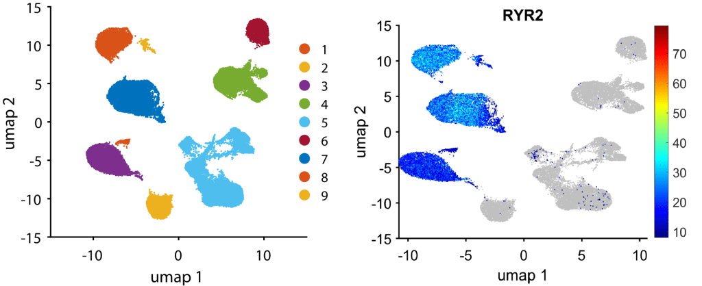
It suggests that clusters 1, 3, 7, 8, 9 are cardiomyocytes.
Also, we can use PlotSampleCellDistribution to view the distribution of cell clusters on UMAP and on the stack bar chart. It is easy to see that cluster 3 is Fetal cardiomyocyte, and cluster 8 is CTL-P56 cardiomyocyte

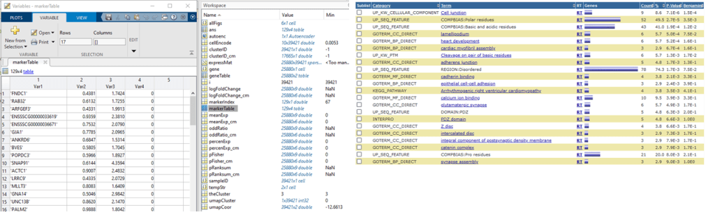
We can view all statistics in cluster 3 and select the marker
theCluster = 3;
% we define the marker for cluster 3: expressing in at least 40% of the genes and cluter fold change > 1.5
markerIndex = find( logFoldChange(:, theCluster) > 1.5 & percenExp(:, theCluster) > 0.4 );
markerTable = table(gene(markerIndex), percenExp(markerIndex, theCluster), logFoldChange(markerIndex, theCluster), pRanksum(markerIndex, theCluster));
The result is in ‘markerTable‘. We can use these genes to analyze enriched pathway and ontologies by DAVID (copy and paste). The result looks like:
IV. Cell cycle analysis using Sparse model
Technically, the results in step 3 allow selecting cluster markers and performing enrichment analysis (i.e. using DAVID david.ncifcrf.gov/). Yet, there are ‘difficult’ cases. For example, the DAVID results above could not tell cycle enriched in fetal-cardiomyocyte. Therefore, we analyze cell cycle using Sparse model analysis. The list of G1S phase markers is in file ‘G1S_Gene.txt’. We will extract an expression matrix that only contains G1S markers and cardiomyocytes. Then, we built the sparse model classifying Fetal and CTL-P56 only using G1S markers.
G1SGeneList = importdata('G1S_Gene.txt');
G1SGeneIndex = find( ismember(gene, G1SGeneList) == 1 );

% get the expression matrix containing only cardiomyocyte and S phase marker
cmCluster = [1, 3, 7, 8, 9]; % we saw before, clusters 1, 2, 7, 8, 9 are cardiomyocytes
cmCellIndex = find( ismember(clusterID, cmCluster) == 1 );
G1S_cm_expression = expressMat (G1SGeneIndex, cmCellIndex);

% also get the cardiomyocyte cell group (sample ID)
cmCellGroup = sampleID(cmCellIndex);

% then perform sparse model analysis. Fetal is the ‘positive’ group, CTL-P56 is the ‘negative’ group
[allCellScore, enrichTable, sparseModel, vioPlot] = sparseModelAnalyis(G1S_cm_expression, cmCellGroup, 'Fetal', 'CTL-P56');
Then, the vioPlot visualize the ‘G1S‘ score among the groups; besides, the enrichment results are in ‘enrichTable‘
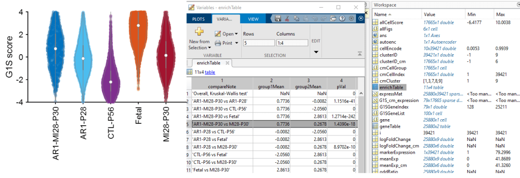
It is clear that Fetal cardiomyocytes have significantly higher score than CTL-P56 ones; also, AR1-MI28-P30 cardiomyocyte scores are significantly higher than the MI28-P30 ones. This result reflects what we expect (and observe) in AR1-MI28 hearts.
Read more
- Nguyen, T.M., Wei, Y., Nakada, Y., Zhou, Y. and Zhang, J., Cardiomyocyte cell-cycle regulation in neonatal large mammals: Single Nucleus RNA-sequencing Data analysis via an Artificial-intelligence–based pipeline. Frontiers in Bioengineering and Biotechnology, p.972.
- Nguyen, T.M., Wei, Y., Nakada, Chen, J., Y., Zhou, Walcott, G., Y. and Zhang, J. Analysis of Cardiac Single-cell RNA-sequencing Data Can be Improved by the Use of Artificial-Intelligence-based Tools. Submitted to Scientific Reports, 2022
- Nakada, Y., Zhou, Y., Gong, W., Zhang, E.Y., Skie, E., Nguyen, T., Wei, Y., Zhao, M., Chen, W., Sun, J. and Raza, S.N., 2022. Single Nucleus Transcriptomics: Apical Resection in Newborn Pigs Extends the Time Window of Cardiomyocyte Proliferation and Myocardial Regeneration. Circulation, 145(23), pp.1744-1747.
