Note: This is the R-replication of the Matlab pipeline in https://github.com/thamnguy/Cardiac-single-cell-AI. The Matlab pipeline is the official one and thoroughly tested. This R-version is primarily to demonstrate the main points in this pipeline; and, hopefully other researcher can re-implement the pipelines in open-source platform. This autoencoder implementation takes more than 1 days to run and requires more than 200GB of memory. We will continue improving the R/Python replication.
I.Overview
This tutorial demonstrates how to use Autoencoder, Sparse model analysis, and semi-supervised learning to analyze single-cell RNA sequencing (scRNAseq) data. Autoencoder is to embed and cluster the cells, and may be repeated multiple times to see novel/interested cell clusters. Sparse model analysis can be used to perform pathway/gene set enrichment analysis, and can also ‘quantify’ the activity of a specific pathway among cell groups. Semi-supervised learning may infer how a specific cell cluster transit to other cell clusters, given that the real-time order is known.
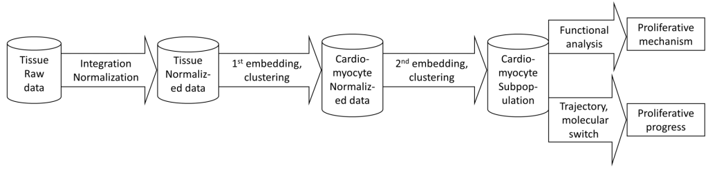
The overall pipeline steps are according to figure 1. It includes
– Data normalization (strongly recommended using Seurat). Also, cell group (sample ID) and expression matrix files need to be processed and slightly formatted
– Cell clustering, embedding, and finding cluster markers. Usually, the first round separates the cell types; then the second and following rounds may identify cell type subpopulations.
– Pathway/geneset enrichment analysis, by Sparse model or marker-based method (i.e. DAVID) – Trajectory analysis can be applied when interesting clusters and time-course information appear.
The dataset used in this tutorial is from https://www.ncbi.nlm.nih.gov/geo/query/acc.cgi?acc=GSE185289. This tutorial only uses the following heart:
Fetal: embryonic day 80 heart. Highly proliferative cardiomyocytes. The code and data for this tutorial can be downloaded at https://uab.box.com/s/0g6r0mauohupfi5e6upxuj3sd7xcfvs6.
CTL-P56: wildtype heart, postnatal day 56. Cardiomyocyte proliferation is virtually 0.
AR1-P28: heart underwent apical resection on neonatal day1, then completely recovered on postnatal day 28
AR1-MI28-P30: heart underwent apical resection on neonatal day1, then the second LAD ligation on day 28. The tissue was collected on postnatal day 30 (2 days after the second injury). It would also completely recover. Cardiomyocytes are expected to proliferate for remuscularization.
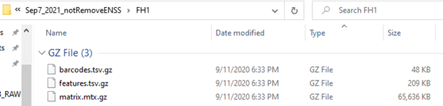
MI28-P30: heart only underwent second LAD ligation on day 28, which would not recover (fibrotic). The tissue was collected on postnatal day 30 (2 days after the second injury). Cardiomyocytes are less proliferative. The raw data, in 10XGenomic format, are supposed to be in the ’10XFormat’ folder. Each group (sample) should have its own subfolder. The 10X format has three files: ‘bardcodes.csv.gz’, ‘features.tsv.gz’, and matrix.mtx.gz’ for each group/sample. For example
II. Data normalization (R/Seurat)
In many cases, Seurat normalization processes the data very well prior to embedding/clustering by Autoencoder. A good Seurat tutorial could be found at https://satijalab.org/seurat/articles/pbmc3k_tutorial.html. The R-Seurat example, which was tested in R version 4.0.3, is below
Step 0: Install the required library (Seurat, sctransform, and Matrix), if needed. Then load them
# install seurat if needed
#install.packages("Seurat")
#if (!requireNamespace("BiocManager", quietly = TRUE))
#  install.packages("BiocManager")
#BiocManager::install("multtest")
# install.packages("autoencoder")
library(Seurat)
library(sctransform)
library("Matrix")library(autoencoder)
Step 1: Import the scRNA data after processed by Cell Ranger. Here we have 5 groups. We would import each group one by one, then merge them into a ‘seuratObj’
Data <- Read10X(data.dir = "10XFormat/Fetal"); seuratObj <- CreateSeuratObject(counts = Data)
Data <- Read10X(data.dir = "10XFormat/CTL-P56");  seuratObj2 <- CreateSeuratObject(counts = Data)
Data <- Read10X(data.dir = "10XFormat/AR1-P28");  seuratObj3 <- CreateSeuratObject(counts = Data)
Data <- Read10X(data.dir = "10XFormat/AR1-MI28-P30");  seuratObj4 <- CreateSeuratObject(counts = Data)
Data <- Read10X(data.dir = "10XFormat/MI28-P30");  seuratObj5 <- CreateSeuratObject(counts = Data)
seuratObj <- merge(seuratObj, y = c(seuratObj2, seuratObj3, seuratObj4, seuratObj5), add.cell.ids = dataID)
rm(seuratObj2); rm(seuratObj3); rm(seuratObj4); rm(seuratObj5); # remove the other 'seuratObj' to free memory
The quality control steps, including removing cells having a high percentage of mitochondrial transcript and doublet detection, are strongly recommended. They are skipped in this tutorial because the data are already processed. See https://satijalab.org/seurat/articles/pbmc3k_tutorial.html for more details in quality controls.
Step 2: Normalize the data with Seurat. This tutorial does not use Seurat’s SCTransform function
seuratObj <- NormalizeData(seuratObj, normalization.method = "LogNormalize", scale.factor = 10000)
seuratObj <- FindVariableFeatures(seuratObj, selection.method = "vst", nfeatures = 2000)
seuratObj <- ScaleData(object = seuratObj, vars.to.regress = c("nCount_RNA", "nFeature_RNA"))
seuratObj <- RunPCA(seuratObj, features = VariableFeatures(object = seuratObj)) # run PCA
seuratObj <- RunUMAP(seuratObj, dims = 1:30, verbose = FALSE) # run Umap
seuratObj <- FindNeighbors(seuratObj, dims = 1:30, verbose = FALSE) # clustering
seuratObj <- FindClusters(seuratObj, verbose = FALSE)
The seuratObj stores the normalization data, which we will need in running Autoencoder.
Step 3: Build the autoencoder
## the autoencoder parameternl=3 ## number of layers (default is 3: input, hidden, output)
unit.type = "tanh" ## specify the network unit type, i.e., the unit's activation function ("logistic" or "tanh")
N.input = seuratObj$RNA@data@Dim[1] ## number of units (neurons) in the input layer
N.hidden = 10 ## number of units in the hidden layerlambda = 0.0002 ## weight decay parameter
beta = 6 ## weight of sparsity penalty term
rho = 0.01 ## desired sparsity parameter
epsilon <- 0.001 ## a small parameter for initialization of weights as small gaussian random numbers sampled from N(0,epsilon^2)
max.iterations = 2000 ## number of iterations in optimizer
## Train the autoencoder
autoencoder.object <- autoencode(X.train=as.matrix(seuratObj$RNA@data), nl=nl, N.hidden=N.hidden,  unit.type=unit.type, lambda=lambda, beta=beta, rho=rho, epsilon=epsilon, optim.method="BFGS",max.iterations=max.iterations, rescale.flag=TRUE, rescaling.offset=0.001)
## Encode / embedd the cells
X_output <- predict(autoencoder.object, X.input=as.matrix(seuratObj$RNA@data), hidden.output=TRUE)
hidden = X_output$hidden.output
