What is a random forest?

Random forests have left the… well, forests of machine learning esoterica and become an analysis technique in nearly every scientific field. In perioperative medicine, this technique has been used to automatically predict patient mortality more accurately than ASA (Hill and colleagues, 2019), blood transfusion needs (Jalali and colleagues 2020), hemorrhage detection (Pinsky and colleagues 2020), and prolonged length of stay (Gabriel and colleagues 2019). But what is a random forest?

Decision tree

To understand the forest, we must first understand the trees. At least, that’s what my meditation app told me this morning. It was a prescient comment because random forests are indeed made up of trees.

Imagine that I asked you if a patient about to undergo surgery is at higher risk of mortality. You might ask me questions like, “What is the patient’s ASA score?” Suppose I say, “2.” Then you might ask about the surgery they’re about to have. Or you might ask me about their age. With each answer, you’re improving your prediction about mortality. And each answer might inform the next question you ask. If I said ASA 3, your second question might be different than if I say ASA 1. Mentally, you are constructing a decision tree to answer my question.

As a visual example, consider if you are trying to decide what kind of room a patient should be placed in based on information from an electrocardiogram. You might use a decision tree like the following.


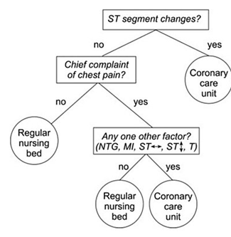
Decision tree example by SilviaCalvanelli. Used with permission under the creative commons CC-BY-SA-4.0 license. This is an illustrative example only. No actionable information is communicated in this figure. It should not be used by anyone for anything.

Now that you have a conceptual understanding of a decision tree, we can return to the idea of random forests.

Random forest

Think about the mortality risk question again. Instead of just asking one clinician, what if I got twenty together in a room and asked them all this question? Obviously, things might get messy if everyone starts asking me about the patient at once. So, in this imaginary scenario, I say that everyone gets to ask one question, and each person must tell me their prediction as soon as their question has been answered. I treat each person’s prediction like a vote, and once all the votes are in, I announce the winning prediction (high risk or not).

With these 20 clinicians each asking one question and getting one vote, I’ve constructed a random forest with 20 trees, each having a maximum depth of 1. If each clinician got to ask 2 questions, then the maximum depth would be 2, and so on. If I had 100 clinicians, then the forest would have 100 trees.

The take away from this example is that a random forest is a whole bunch – potentially thousands – of very simple models that are each allowed to ask only a few questions before making a prediction. The votes from all the simple models are then tallied, and the winning prediction is announced. The technique sometimes seems comically basic, but random forests have proved to be powerful prediction tools.

Notes

The example above certainly isn’t perfect. In a more precise example, the trees wouldn’t directly know each other’s questions, but they would be told whether their answer was improving the prediction based on cases where we already know the right answer, and they would be allowed to change their questions and votes accordingly. This process is called “model training.” Also, each tree wouldn’t start from a place of expert knowledge – like clinicians would – these would be more like randomly selected non-medical folks who were given a list of potential questions to choose from.  Finally, the final prediction doesn’t have to be a majority vote. As an alternative, each participating could say how confident they are in their answer, and then the average confidence could be used to pick the winning answer.

References

Hill, B. L., Brown, R., Gabel, E., Rakocz, N., Lee, C., Cannesson, M., Baldi, P., Olde Loohuis, L., Johnson, R., Jew, B., Maoz, U., Mahajan, A., Sankararaman, S., Hofer, I., & Halperin, E. (2019). An automated machine learning-based model predicts postoperative mortality using readily-extractable preoperative electronic health record data. British Journal of Anaesthesia, 123(6), 877–886. https://doi.org/10.1016/j.bja.2019.07.030

Gabriel, R. A., Sharma, B. S., Doan, C. N., Jiang, X., Schmidt, U. H., & Vaida, F. (2019). A Predictive Model for Determining Patients Not Requiring Prolonged Hospital Length of Stay after Elective Primary Total Hip Arthroplasty. Anesthesia and Analgesia, 129(1), 43–50. https://doi.org/10.1213/ANE.0000000000003798

Pinsky, M. R., Wertz, A., Clermont, G., & Dubrawski, A. (2020). Parsimony of hemodynamic monitoring data sufficient for the detection of hemorrhage. Anesthesia and Analgesia, 130(5), 1176–1187.

Jalali, A., Lonsdale, H., Zamora, L. V., Ahumada, L., Nguyen, A. T. H., Rehman, M., Fackler, J., Stricker, P. A., & Fernandez, A. M. (2020). Machine Learning Applied to Registry Data. Anesthesia & Analgesia, Publish Ahead of Print(Xxx), 1–12. https://doi.org/10.1213/ane.0000000000004988

More p-values, more problems

I’m a fan of the web comic XKCD by Randall Monroe, which takes esoteric math and science concepts and turns them into jokes. In one edition, Monroe tackles the issue of multiple hypothesis testing: If you test many hypothesis simultaneously without adjusting your significance cutoff (e.g., p<0.05), false positives are going to happen more than you might expect.

In the related edition of XKCD, two characters want to know if jelly beans cause acne. Scientists investigate this claim and find no link between jelly beans and acne. That is, the scientists test the null hypothesis, “There is no statistically significant relationship between jelly bean consumption and acne.” The results will not surprise you.

XKCD “Significant” panels. Used under creative commons license CC BY-NC 2.5.

In this joke example, the scientists test one hypothesis, calculating one p-value and comparing that one p-value to a critical value (here 0.05). No problem so far. But, what if I am concerned that one specific color out of a possible, say, 20 jelly bean colors causes acne?

XKCD “Significant” panels. Used under creative commons license CC BY-NC 2.5.

So green jelly beans cause acne? I can see the headlines now.

XKCD “Significant” panels. Used under creative commons license CC BY-NC 2.5.

Notice that part of this joke front-page news there is a comment “only 5% chance of coincidence.” Is that right? If the scientists had tested a single hypothesis, then yes. However, that’s not what happened. The scientists tested 20 hypotheses. So what are the odds this result happened by chance?

Remember that a p-value tells you the likelihood of getting a result as extreme or more extreme by chance. That means for a single hypothesis test, the p-value tell you the likelihood of getting something like your result by chance. What about if I tested 20 independent hypotheses with a cutoff of 0.05? In that case,

There is a 64% chance of at least one false positive. Said another way, it is more likely than not that this experiment will yield at least one false positive just by chance.

What do we do?

The simplest approach is to divide your cut off value by the number of simultaneous hypotheses (Miller 1981). This process is called a Bonferoni correction In this case, that would be

You may think, “That’s a very strict cutoff.” You’re right. This cutoff will do a great job of preventing false positives. In fact, we can prove it.

This number, 0.0488, can be thought of as the cut-off equivalent. If we were to somehow condense all 20 tests into 1, the cutoff for this test would be 0.488. However, as you might expect, this process results in more false negatives than would be expected from a single hypothesis test. In fact, you can prove that the false negative rate tends toward 1 as the number of tests increases (Efron 2004). That is, if you do a lot of simultaneous tests with this method, you’ll fail to reject the null hypothesis nearly every time, regardless of whether there is actually a relationship in your data.

The Bonferoni correction is still useful, though. If having even one false positive would mean disaster for your work, then the Bonferoni correction may be the way to go, as it is quite conservative. Likewise, if you are testing only a small number of hypotheses (say <25) and you expect (based on prior knowledge) that only one or two are true, the Bonferoni correction may be the way to go.

There are other options. I’ve linked to resources on a few below, but I would suggest reaching out to a Data Scientist for a consultation on what the best option is for your particular research project.

One option is to control the False Discovery Rate (FDR). For a practical guide to this process, see the section “Controlling the false discovery rate: Benjamini–Hochberg procedure” on this external blog post.  For a theoretical description, see Benjamini and Hochberg 1995.

Another option that has shown promise in Anesthesia and Analgesia literature (double meaning intended) is to re-frame your hypotheses to do joint hypothesis testing or a “gate keeping” procedure where you test a second hypothesis under the condition that the first is true (Mascha and Turan 2012).

You can also calculate Benjamini–Hochberg adjusted p-values, sometimes called q-values in some statistical software. However, these adjusted p-values lack the theoretical backing of typical p-values and methods for controlling FDR. They can be useful for quick-and-dirty analysis, but they should be avoided for publication purposes. A careful reviewer may object that such q-values lack statistical rigor. If you want to learn more about these adjusted p-values, these Berkeley lecture notes provide a succinct guide.

References

Munroe, Randall. “Significant.” XKCD. https://xkcd.com/882/.

Miller, R. (1981), Simultaneous Statistical Inference (2nd ed.), New York:
Springer-Verlag.

Efron, B. (2004). Large-scale simultaneous hypothesis testing: The choice of a null hypothesis. Journal of the American Statistical Association, 99(465), 96–104.

Mascha, E. J., & Turan, A. (2012). Joint hypothesis testing and gatekeeping procedures for studies with multiple endpoints. Anesthesia and Analgesia, 114(6), 1304–1317.5

Benjamini, Yoav, and Yosef Hochberg. “Controlling the false discovery rate: a practical and powerful approach to multiple testing.” Journal of the Royal statistical society: series B (Methodological) 57.1 (1995): 289-300.

A risk scorecard for COVID-19

A product of the UAB COVID-19 Data Science Hackathon

On June 15 and 16, I participated in the UAB COVID-19 Data Science Hackathon. My teammates and I created a scorecard model and web app that predicts the likelihood of an individual being infected with COVID-19 based on demographics, pre-existing conditions, and symptoms. We were one of three teams to win a cash prize in the competition for the novelty and success of our work.

My teammates were Thi K. Tran-Nguyen, Tarun Karthik Kumar Mamidi, and Liz Worthey (who proposed the question we focused on). Together, our skills covered the gamut of data wrangling, model development, and medical relevance. As a result, we developed a proof of concept model and web app that we envision could be used by a broad population including both patients and providers. The end result is like looking at your credit score, except that it tells you if you are at higher risk of having COVID-19.

Scorecard web app demo prepared by Tarun Mamidi.

This work may be of particular interest to perioperative medicine for both specific patient screening for COVID-19 and risk stratification methods in general.

The hackathon showcase presentations were recorded on Friday, June 19, 2020. To view the presentation for this visit, click here.